Transforms
Transforms
Graph transformation is a central concept in Graphia. Transforms are a range of processes by which a graph is modified to produce a new graph or calculate a new attribute. Graphia incorporates a wide range of options that allow an analyst to perform a sophisticated range of data transformations and analyses. These include processes such as graph clustering, edge reduction, node/edge filtering based on attributes, calculation of graph metrics, or algorithms that change the structure of a graph. Graphia’s interface for performing graph transforms has been designed to be powerful and flexible, the results immediately modifying a graph’s structure or appearance.
The Add Transform button can be found in the top right of the graph view. From here a list of transforms can be selected (see below).
Active transforms are displayed in a list on the top right of the graph display. Transforms are applied top down; the transform at the top of the list is applied first, the results of which are then fed into the second transform and so on down the list. The result of this process is what is ultimately displayed.
![]()
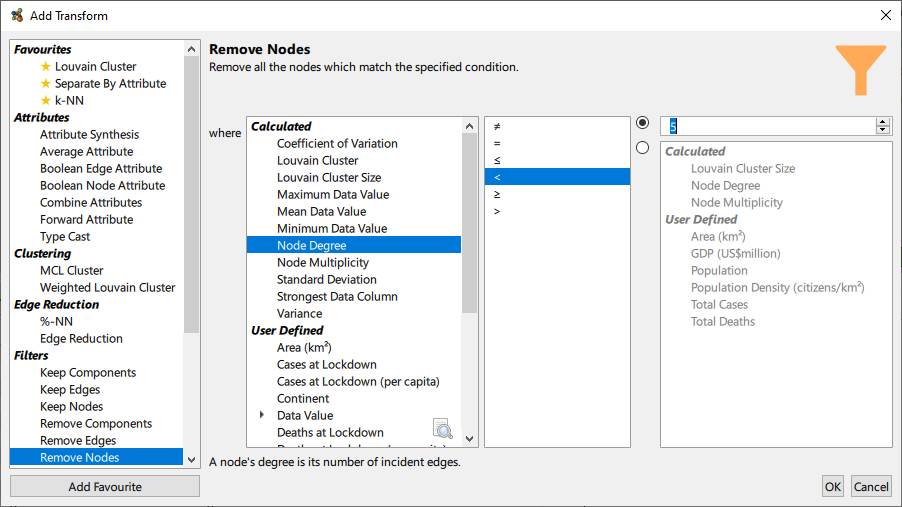
Clicking Add Transform will bring up the following dialog:
![]()
From here you are presented with a list of all transforms available, separated by category. Selecting a transform from the list will elicit a brief description of the transform and its associated parameters.
- Attributes: modify or add new attributes using the values of existing attributes
- Clustering: partition the graph into distinct clusters
- Edge reduction: globally reduce the number of edges in a graph, while approximately maintaining structure
- Filters: conditionally filter elements based on their associated attributes
- Metrics: introduce new attributes that measure elements’ placement within the graph
- Structural: change the structure of a graph in various ways
Some transforms provide the option to automatically apply a visualisation after adding. Transforms that are used often can be set as favourites using the Add/Remove Favourite button. In this case such transforms will always appear at the top of the list, for easy access. Clicking OK will finalise the transform configuratiom and add it to the graph. We describe some of the most commonly used transforms below.
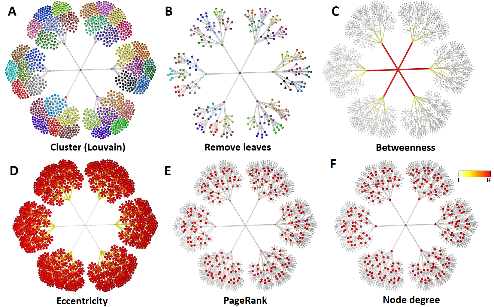
Clustering
Clustering is the act of dividing a graph up into groups of nodes based on their position within the overall topology of the graph. These are referred to as clusters. Clustering seeks to divide the graph into communities that are likely to possess similar properties or characteristics. Graphia incorporates two of the most widely used algorithms for performing this analysis, the Markov Clustering (MCL) and Louvain clustering algorithms. Both include the option to change the granularity of clustering, i.e. how many clusters are formed. There is no simple answer to the question of what the correct clustering of a graph is, but good visualisation allows one to look at the results of a cluster analysis and how it maps on to a graph’s structure. Once data has been clustered, clusters can be analysed by enrichment analysis to see if there are any node attributes over-represented within the groups.
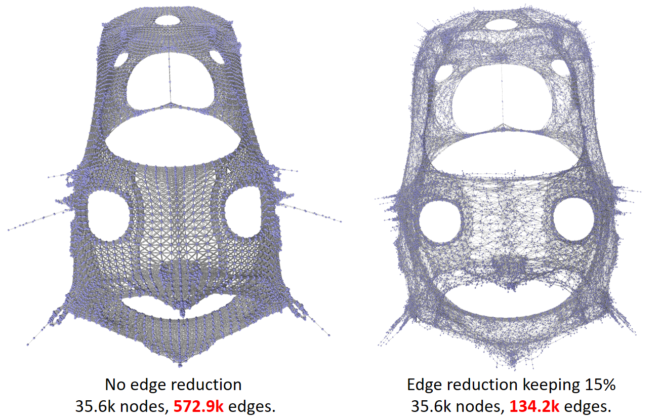
Edge Reduction
In some graphs the number of edges can be exceptionally large. Not only can these be difficult to render, they may add little to the overall structure and can actually obscure higher level groupings. The k-nearest neighbours (k-NN) algorithm is widely used for globally reducing the number of edges in a graph, such that a given node has a maximum number of edges. In a weighted edge graph it is preferential to retain those with the strongest weights. A modification of this principle is to retain only a given percent of the edges for any given node (%-NN). In the case where there are no edge attributes available there is also the option to remove a homogenous sample of the edges (Edge Reduction transform).
Filters
The filter transforms allows a user to remove nodes or edges based on their attributes. It provides a functionally rich menu with which to transform a graph based a wide range of criteria.
Metrics
Graphia includes three metrics for analysing a graphs structure:
- Betweenness: centrality is a measure of centrality in a graph based on the shortest paths between nodes. The betweeness centrality is the number of these shortest paths that pass through the node.
- Eccentricity: calculates the shortest path between every node and assigns the longest path length found for each node. This is a measure of a node’s position within the overall graph structure.
- PageRank: is an algorithm used originally to measure the importance of website pages. PageRank works by counting the number and quality of links to a page to determine a rough estimate of how important a node is.